LiDARSnap Tuning and Parameters

Some commonly used LiDARSnap terminology is defined here.

Correspondences

Correspondences are LiDARSnap's primary source of input information. A correspondence is a pair of surfaces in the pointcloud that have a similar orientation and position. Correspondences occur where data recorded at different times overlap spatially. In the case of aerial data, correspondences are found in the overlap area between flightlines.

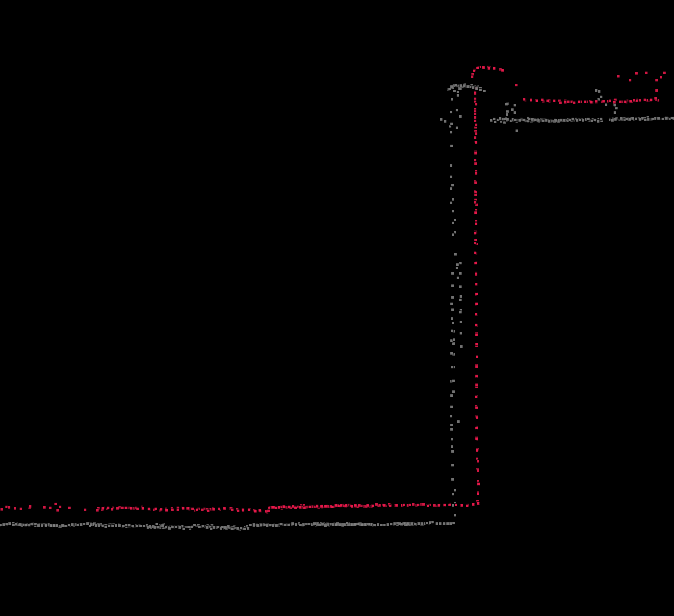
Ex. 1: A pointcloud is visualized by interval (flightline). Two intervals overlap on the same wall. LiDARSnap would likely identify at least two correspondences (one for the ground surface, and one for the wall surface):

Two flightlines overlapping on a building wall. This data is uncalibrated. LiDARSnap would observe correspondences on the wall and ground surface, and then use the correspondences to solve for trajectory or sensor parameters.

Single pass data cannot be processed by LiDARSnap, because there is no spatial overlap to the lidar data and thus correspondences cannot be found.

Sampling Radius

LiDARSnap searches for correspondences at radius specified by this parameter. Reducing this parameter results in more detected correspondences, but slower processing times. Increasing this parameter may be necessary with large (> 10 km^2) data sets, to prevent from over-consuming computer temporary space (all correspondences must be stored in temp space, specified in Local Settings->Processing->Temporary Storage).

Normal Search Radius

As mentioned above, two surfaces are only considered a correspondence if they both face the same direction. The direction of the surface is determined by computing a surface normal. The surface normal is a vector that is orthogonal to the computed surface.

A two lane road is used to visualize surface normals. Normals on the road point up (90 degree elevation angle), whereas normals detected on tree trunks point out to the left or right (0 degree elevation angle).
The normal search radius is the size of the area used to compute the surface normal. With large features, such as a road surface, the surface normal computed is the same whether a 0.10 m or 2.0 m normal search radius is used to compute the normal. With smaller features, such as a pole or tree trunk, it's important to compute the normal vector using an area that will accurately capture the surface. In the example above, a 0.10 m normal search radius was used, to ensure that normals were observed on tree trunks.

If a group of points does not have a clear surface normal, this surface is discarded. A good example of this is in the tree canopy, where points in the tree canopy occur in a somewhat random fashion. When a normal is computed for this region of points, it's roughness is considered high.

Residuals

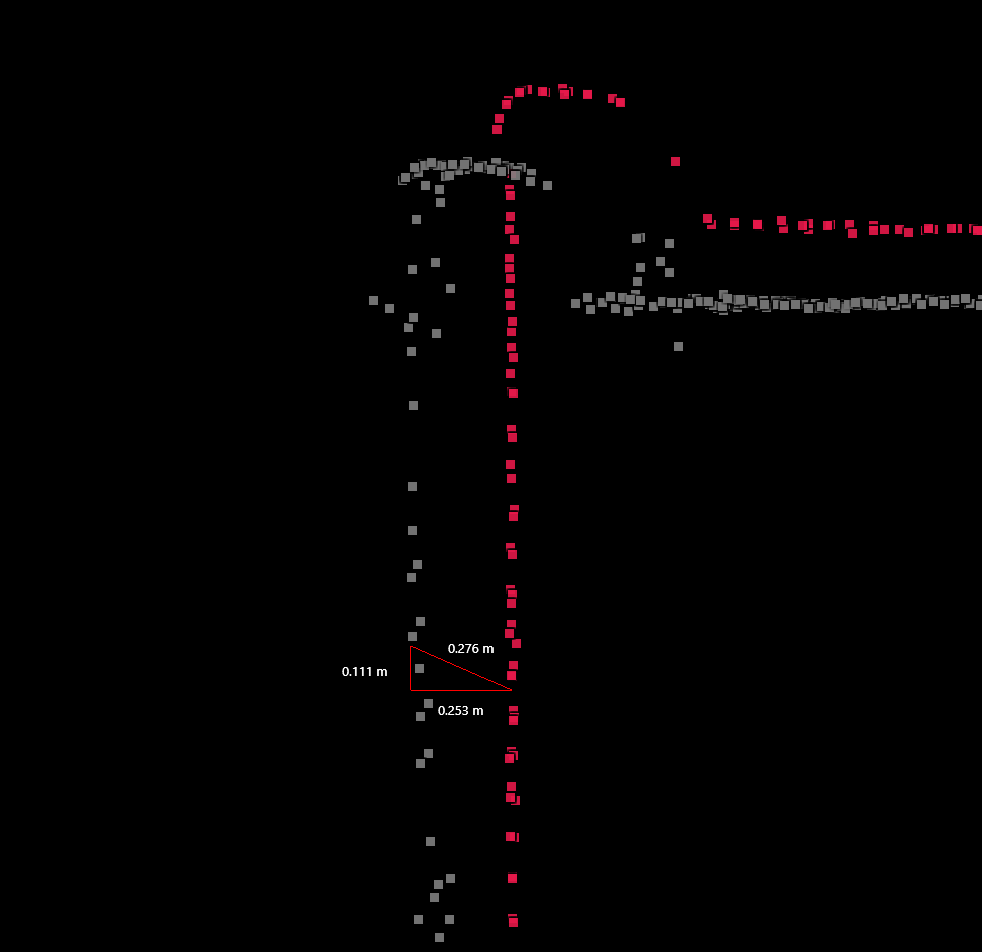
A residual is the distance between the two surfaces in a correspondence. LiDARSnap's goal is to reduce residuals. In the example above, where a correspondence is detected on a wall, the pre-optimization residual would be about 25 cm:

After optimization, the residual is much less:

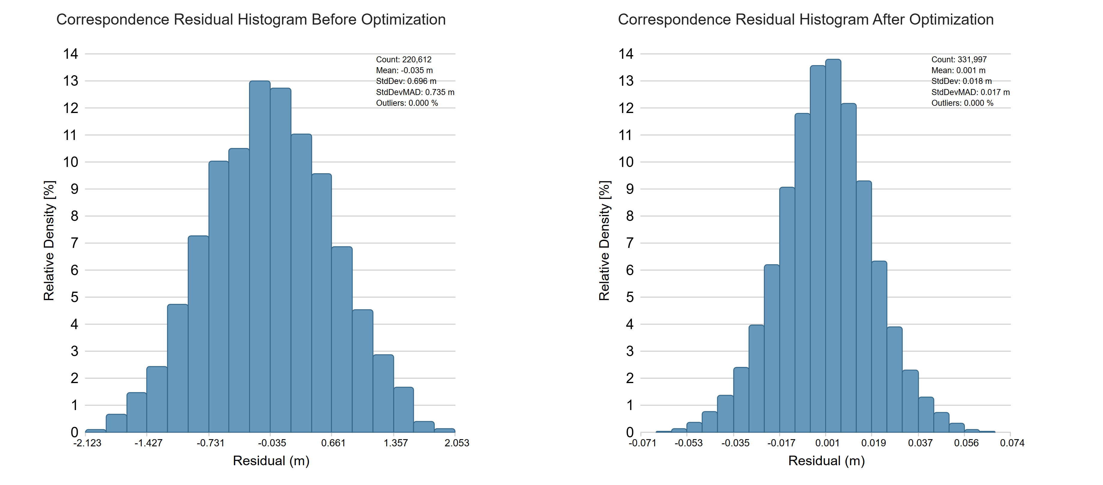
The LiDARSnap report shows histogram distributions of residuals before (left) and after (right) optimization:

Whether residuals are positive or negative is somewhat arbitrary, as it depends on which direction is considered positive/negative. After optimization via LiDARSnap, the residuals should follow a gaussian distribution around a mean of zero. One of the most useful metrics of LiDARSnap's success is the standard deviation of the residuals (shown on the plot as StdDev). This conveys the typical magnitude of residuals after optimization, which in the plot about is about 0.018 m.

Last updated